Contents
- Introduction
- Optimizing a FastAPI Trace Ingestion Server for LLM Observability
- Results
- Conclusion and Learnings
- Reflection
Introduction
Recently, I had an exciting final-round interview experience in San Francisco. The task was presented to me on the spot at the company's office and I had no prior exposure to the codebase or the problem domain. My challenge was to optimize a simplified implementation of a FastAPI-based server designed for ingesting batches of trace data ("runs") for an observability platform tailored for LLM applications.
The provided implementation was slow and memory-intensive, suffering from inefficient database operations, redundant JSON serialization, and multiple sequential S3 uploads. Within just a few hours, I was able to improve the performance by identifying key bottlenecks by introducing connection pooling, batching database inserts, parallelizing and streaming S3 uploads, adding caching, and refining the data schema which ultimately helped improve the trace ingestion pipeline around 6x faster while reducing memory usage.
Although I didn't secure the position, the experience was highly rewarding, allowing me to tackle an engaging technical challenge, learn valuable lessons, and interact with inspiring engineers.
Optimizing a FastAPI Trace Ingestion Server for LLM Observability
TL;DR
I improved the performance of a FastAPI-based trace ingestion server, significantly reducing processing time and memory usage through strategic optimizations.
| Scenario | Before (mean sec) | After (mean sec) | Improvement |
|---|---|---|---|
| 500 runs (10KB each) | 2.13s | 0.35s | ~6x faster |
| 50 runs (100KB each) | 0.56s | 0.20s | ~2.8x faster |
Project introduction
I was given an API server built with FastAPI that accepts batches of “runs”, basically they're JSON objects representing trace events emitted by LLM-powered agents. Each run captures a single unit of trace data, including details like the input prompt, the model's output, metadata (such as timestamps, model type, and identifiers), and other invocation context. A batch might include dozens or hundreds of these runs, often totaling several megabytes of data.
In production, these batches would be sent in rapid succession, especially under high load. The observability system needs to ingest them quickly, persist them efficiently, and respond with minimal latency. My task was to improve the throughput and memory efficiency of this ingestion process of the current system that they'd provided by optimizing how these batches are handled, stored, and acknowledged by the server.
Here's an example of what a single run looks like:
{
  "id": "2f5b8e22-8c3f-4d3b-9a5d-1d2e9e0f7abc",
  "trace_id": "f1e9d5c3-1234-4a1b-b567-8d0c9a0e1def",
  "inputs": { "prompt": "Hello, world!" },
  "outputs": { "response": "Hello to you!" },
  "metadata": { "model": "gpt-3.5-turbo", "timestamp": "2025-03-01T12:00:00Z" }
}
A batch of runs is simply a list of many such JSON objects (the batch could be dozens or hundreds of runs, potentially totaling several MBs of data).
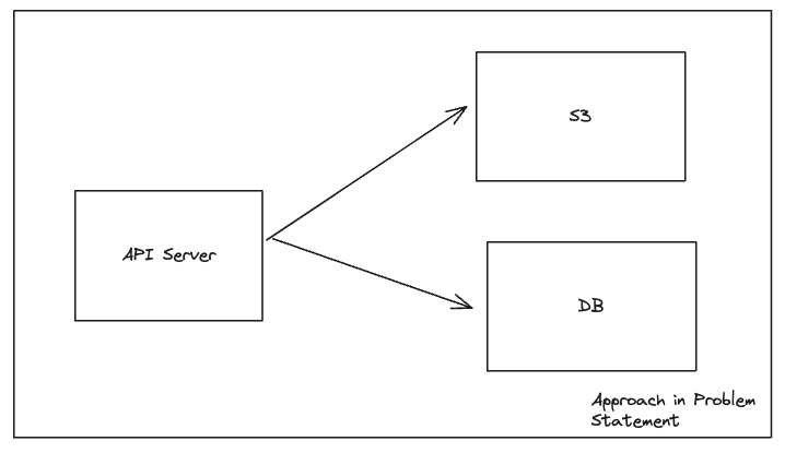
Initially, the server stored each run's data in a Postgres database (including the large inputs/outputs fields as text) and also uploaded the run details to an S3 bucket for backup and retrieval. The goal of this project was to improve the throughput and memory efficiency of this ingestion process, especially for large batches.
This is how (roughly) the initial API server that I was given, functioned:
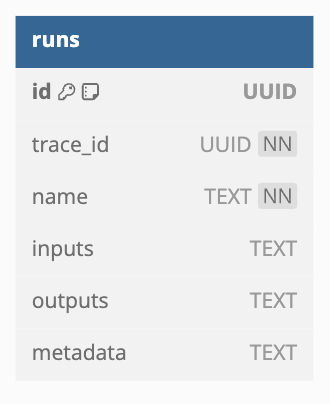
This is the initial database schema that I was given:
Benchmark Summary
To gauge performance, I was given benchmark tests for two scenarios:
- 500 runs @ 10KB each: Simulates a batch of 500 small runs (each run's JSON roughly 10 KB in size, total ~5 MB).
- 50 runs @ 100KB each: Simulates a batch of 50 larger runs (each ~100 KB, total ~5 MB as well). The measurement was the time taken to process each batch in the baseline vs. the optimized implementation.
In the “500x10KB” case, mean latency dropped from ~2.13 s to ~0.35 s, and in the “50x100KB” case from ~0.56 s to ~0.20 s. As we can see, the optimizations led to 6x faster processing for the 500-run scenario and about 2.8x faster for the 50-run scenario. In both cases the total payload is ~5 MB, but the baseline struggled more with many small runs (overhead per run), which is why the improvement there is especially large. The final implementation not only handles more requests per second, but also uses less memory and CPU per batch.
Deep Dive into the Engineering Journey
Analyzing Baseline Performance
I began by writing dedicated benchmark tests and profiling the application to uncover hot spots. The initial analysis revealed a few major issues:
- High memory usage during serialization: Converting Python objects to JSON (using orjson.dumps) for each run was consuming a lot of memory and CPU, especially for big batches. The server would construct large JSON strings (sometimes several MB) entirely in memory before sending to S3, causing memory spikes.
- Inefficient S3 uploads: Runs were being uploaded to S3 one by one. For a batch of hundreds of runs, this meant hundreds of separate S3 PUT operations. Moreover, all the run data was held in memory as large strings during upload. This resulted in excessive network overhead and memory pressure.
- Inefficient database access: Database inserts were performed individually for each run, with a fresh transaction each time. In other words, the code was looping through runs and doing
INSERTqueries one-by-one. This is slow due to round-trip overhead and lacked any form of bulk operation. Also, the database connection was not being reused effectively (no connection pooling), meaning new connections or cursors were created frequently. - Suboptimal data retrieval design: The original schema stored large JSON blobs (inputs, outputs) directly in the runs table, which made read queries heavy. Even after introducing S3 for storage, retrieving a run meant joining the runs metadata with the S3 key and then fetching from S3, which was not optimized.
Using these findings, I set out to address each problem systematically. Here's a pseudocode version of the naive implementation I was asked to optimize. It uses synchronous operations and lacks pooling or batching, but helps illustrate the underlying issues:
# Original naive implementation (simplified):
def create_runs(batch_of_runs):
    # No connection pool: open a new DB connection for this batch
    # illustrative only: no pooling, sync operations
    conn = connect_to_postgres(DB_CONNECTION_STRING)
    cursor = conn.cursor()
    s3_client = connect_to_s3() # S3 client (could be re-created each time)
    for run in batch_of_runs:
        # Insert run into database (inputs/outputs stored as text in DB)
        cursor.execute(
            "INSERT INTO runs (id, trace_id, inputs, outputs, metadata) VALUES (%s, %s, %s, %s, %s)",
            (run["id"], run["trace_id"], json.dumps(run["inputs"]), json.dumps(run["outputs"]), json.dumps(run["metadata"]))
        )
        conn.commit()  # committing inside the loop (very slow!)
        # Serialize run data to JSON (into memory)
        run_json = orjson.dumps(run)
        # Upload to S3 (one request per run)
        s3_client.put_object(Bucket=RUNS_BUCKET, Key=f"runs/{run['id']}.json", Body=run_json)
    cursor.close()
    conn.close()
    return {"status": "ok"}
In short, this version
- opened a fresh DB connection per request
- committed inside the loop
- serialized each run individually
- made a separate S3 PUT call for every run. All of this resulted in excessive round-trips, redundant memory usage, and poor scalability under large batch sizes.
Now that we've established the problems with the initial implementation, let's dive into the changes I made to the code to address these issues.
Note: All code snippets in this post are illustrative and rewritten to avoid any NDA violations. They reflect the engineering approaches I took, but are not lifted from the actual source.
Added Connection Pooling for the Database
The first improvement was to enable connection pooling for the Postgres database. Without pooling, each request (or each iteration) had to establish a new DB connection, which is expensive. I implemented a custom class to help manage a connection pool so that connections could be reused across requests. The idea behind this was to avoid the overhead of repeatedly opening/closing connections and also helps the database handle concurrent requests more smoothly.
Here's an equivalent snippet using SQLAlchemy-style pooling for illustration, though my actual implementation used asyncpg with a custom pool manager:
# At app startup
engine = create_engine(DB_DSN, pool_size=10, max_overflow=5)
SessionLocal = sessionmaker(bind=engine)

# In request handler
session = SessionLocal()  # this reuses a connection from the pool
# ... use session to insert runs ...
session.commit()
Switching to pooled connections reduced average latency variability and eliminated delays observed when opening fresh connections under load.
It was a necessary foundation for the next improvements. (Note: S3 connections were already being handled via an aiobotocore session under the hood. The aiobotocore session factory creates reusable clients with built-in connection reuse)
Summary of wins with connection pooling:
- Eliminated overhead from repeatedly creating TCP connections
- Reduced tail latencies during burst traffic
- Allowed safe reuse across coroutine calls
Batched Inserts to Postgres
The next major win was changing how I performed database inserts. Doing separate INSERT queries for each run is far from optimal. I refactored the code to perform bulk inserts in a single transaction. There are two techniques that I tried:
Technique 1: Single transaction, multiple inserts. (I used this technique)
Instead of committing inside the loop for each run, I accumulate all the new run records and commit once at the end. Using an ORM (like SQLAlchemy), this could mean adding all run objects to the session, then one session.commit(). If using raw SQL, it could mean issuing one multi-row INSERT (or using executemany). This drastically reduces transaction overhead.
Technique 2: Bulk insert helpers from ORMs
I leveraged SQLAlchemy's bulk insert feature (session.bulk_insert_mappings or session.bulk_save_objects) to efficiently insert all runs in one go. These bypass some of the ORM overhead and directly insert multiple rows.
For example, using SQLAlchemy's Core or Psycopg2 directly:
# Using psycopg2 to do batch insert
records = [(run["id"], run["trace_id"], json.dumps(run["name"])) for run in runs]
cursor.executemany(
    "INSERT INTO runs (id, trace_id, name) VALUES (%s, %s, %s)",
    records
)
conn.commit()
If the runs table doesn't include the large inputs/outputs fields anymore (more on this later), the insert is lightweight. In our optimized code, I removed those large text fields from the runs table entirely and only insert metadata and identifiers, which is very fast(because we're just dealing with some strings). By batching the inserts, the database can handle the load in a single transaction. While testing this change it yielded a significant boost. The benchmarks showed that moving from per-run commits to one bulk commit was one of the biggest contributors to the speedup. I went from hundreds of small writes to a single set of writes, cutting down the overhead significantly.
Crucially, handling the entire batch within a single database transaction ensures atomicity. This 'all-or-nothing' property guarantees that either all runs in the batch are successfully persisted, or none are if an error occurs mid-batch. This not only protects against partial writes but also simplifies debugging and downstream consistency so that if the batch fails, we know nothing was written.
Summary of wins with batched inserts:
- Reduced transaction overhead by replacing per-run commits with a single atomic transaction per batch
- Improved throughput and database efficiency by placing all inserts inside a single transaction block per batch
- Minimized ORM overhead, maintaining tight control over SQL execution paths
- Ensured data consistency and atomicity, preventing partial writes and making error handling cleaner
Improved Schema and Added Indexes
This was the given schema at the beginning:
-- runs - this is the schema that I started with
CREATE TABLE runs (
    id UUID PRIMARY KEY DEFAULT gen_random_uuid(),
    trace_id UUID NOT NULL,
    name TEXT NOT NULL,
    inputs TEXT,
    outputs TEXT,
    metadata TEXT
);
I realized that part of the slowness was due to the way data was modeled in the database. The original runs table stored large JSON blobs (inputs, outputs, metadata) in each row, which was not only slow to insert but also not needed since I was putting that data in S3. I decided to redesign the schema for efficiency:
-
I removed large blob columns from the runs table. In a migration, I dropped the inputs, outputs, and metadata text columns, since the detailed data would be in S3. This made each run record much smaller (just IDs, timestamps, etc.).
-
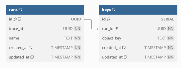
I introduced a separate keys table to store S3 object keys for each run. Each entry in keys links a run_id to an object_key (the S3 key where that run's data is stored). This helped normalize the design and clearly separated metadata (frequently queried) from large blobs (rarely queried), with the latter delegated to S3 for cold storage. After this change, saving a run to the DB meant inserting a row into runs (small and fast) and a row into keys (also small). No more large text fields in the DB. The heavy lifting (storing the actual input/output data) is delegated to S3.
-
I also added indexes to speed up queries, especially for retrieving or filtering runs:
- An index on
runs.trace_id` helps to query all runs belonging to the same trace (common in observability when showing a full trace timeline) - An index on
runs.created_atwas added to quickly sort or range-query runs by time. - Indexes on the keys table for
run_idandobject_keyto expedite joins and lookups.
- An index on
These indexes ensure that joining runs with keys to find a run's S3 object, or finding all runs for a trace, are fast operations. Below is the SQL script illustrating some of these schema changes:
-- Updated `runs` table
CREATE TABLE runs (
    id UUID PRIMARY KEY DEFAULT gen_random_uuid(),
    trace_id UUID NOT NULL,
    name TEXT NOT NULL,
    created_at TIMESTAMP WITH TIME ZONE DEFAULT now() NOT NULL,
    updated_at TIMESTAMP WITH TIME ZONE DEFAULT now() NOT NULL
);

-- Indexes on `runs` table
CREATE INDEX idx_trace_id ON runs(trace_id);
CREATE INDEX idx_created_at ON runs(created_at);

-- New `keys` table
CREATE TABLE keys (
    id SERIAL PRIMARY KEY,
    run_id UUID NOT NULL REFERENCES runs(id) ON DELETE CASCADE,
    object_key TEXT NOT NULL,
    created_at TIMESTAMP WITH TIME ZONE DEFAULT now() NOT NULL,
    updated_at TIMESTAMP WITH TIME ZONE DEFAULT now() NOT NULL
);

-- Indexes on `keys` table
CREATE INDEX idx_run_id ON keys(run_id);
CREATE INDEX idx_object_key ON keys(object_key);
Quick Note: I also considered adding some unique constraints on the tables to help with consistency, but since we're not dealing with problems around idempotency, I decided against it.
By separating concerns (keys and runs) and adding these indexes, I'd think helped improve both write and read performance. We didn't have fields that were storing redundant data, and the indexes helped speed up the queries. In fact, after this change, most writes became DB-light (just small inserts).
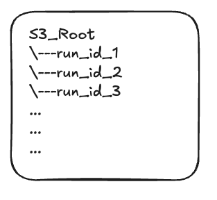
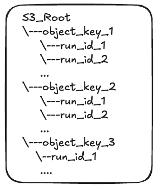
Another impact this had was on the way we stored data in S3. In the initial design we were just storing the data in S3 as JSON file for each run based on the id (or run_id, I use it interchangebly since it helps make the reasoning more clear). But now that we'd established two table, namely runs and keys, for each new batch of runs that we'd receive, we'd generate a random UUID for the batch and create a prefix for it in S3. Then for each run in the batch, we'd store it in the prefix created for the batch. This helped both in terms of organization (because now, tracing of the runs is easier) and IO efficiency which in turn it helped with searchability.
Just to give you a sense of how this looks like, here's a diagram of the S3 bucket when we started out:
And here's a diagram of the S3 bucket after the changes:
Summary of wins with Improved Schema and Added Indexes:
- Reduced row size in the primary runs table by offloading large JSON fields to S3
- Improved insert throughput
- Separated “hot” metadata from “cold” payloads
- Added targeted indexes (trace_id, created_at, object_key)
- Enabled batch-based S3 prefixing, improving traceability of runs
Here's another quick note about something that I'd thought of:
I briefly considered creating a materialized view that pre-joins the runs and keys for even faster reads. However, given the frequent writes, I was worried a materialized view would have maintenance overhead and could lag behind, so I decided against this complexity.
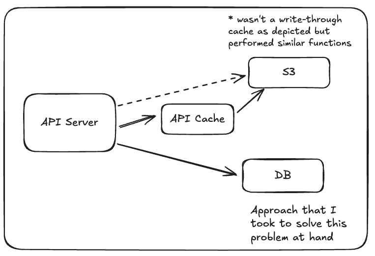
Introduced an API Caching Layer
Even with faster writes, retrieving runs (especially recently written ones) could be slow if I always had to hit S3 for the full data. To mitigate this, I implemented a simple in-memory cache for "run" data. The idea was to store the most recently accessed or created runs in the cache so that if they are requested again shortly after it'd be trivial to serve them quickly without another call to S3.
I implemented an in-memory cache keyed by run ID. This cache is per-process and not shared across instances, which is fine for a single-node deployment or a dev/test setup. In a multi-instance setup, you'd likely need Redis or another shared cache. Whenever a run is ingested, I put its data (the inputs/outputs JSON) into the cache. Likewise, when a client requests a run, I first checked the cache; if it's a hit, I return the data immediately, if not I fetch from S3 and then store it in the cache. I kept the cache size modest and implemented a simple TTL (time-to-live) eviction policy so it doesn't grow unbounded. Newly ingested runs are proactively cached, and any cache misses on read paths populate the cache as a side-effect of a successful S3 fetch, helping "warm" the cache organically.
Example of how this looks in code:
from cachetools import LRUCache, TTLCache

# Cache for runs: up to 1000 entries, evict after 5 minutes
run_cache = TTLCache(maxsize=1000, ttl=300)

def get_run(run_id):
    # Try cache first
    data = run_cache.get(run_id)
    if data:
        return data  # cache hit
    # Cache miss: fetch from S3 (and maybe DB for metadata)
    run_obj = fetch_run_from_s3(run_id)
    run_cache[run_id] = run_obj  # store in cache
    return run_obj
By doing this, if a client immediately requests the run they just submitted (which is common in some workflows), the server can return it without hitting S3 or the DB at all. Similarly, if a trace is being actively viewed (accessing multiple runs), many of those runs will be cached. The cache significantly improved the read performance and reduced repeated work. It's essentially leveraging temporal locality of reference.
The trade-off here is memory usage (locally) since we're using RAM to store some recently used runs. Although I'd set conservative limits to avoid memory bloat. The cache TTL and size were tuned so that it improves speed without consuming too much memory.
Upon adding the cache, the service functioned like so:
Summary of Wins with the API Caching Layer:
- Reduced latency for hot-path
GET /runs/:id- Avoided redundant S3 and DB calls
- Massive improvement in the performance since the cache is doing the heavy lifting
Optimized Batched and Streamed Uploads to S3
Initially, the ingestion server uploaded each run to S3 individually which resulted in hundreds of sequential S3 PUT operations per batch. This led to high network overhead and excessive memory usage, as each run was serialized and buffered in full before upload.
To eliminate this bottleneck, I replaced per-run uploads with a single, streamed batch upload. Instead of creating one large JSON string in memory, I used an async generator to serialize and stream each run directly to S3 as it's being processed.
Here's a simplified version of how the streaming upload works:
async def generate_bytes(run_dicts):
    yield b"["
    for idx, run in enumerate(run_dicts):
        if idx > 0:
            yield b","
        yield orjson.dumps(run)
    yield b"]"

await s3_client.put_object(
    Bucket=settings.S3_BUCKET_NAME,
    Key=f"batches/{batch_id}.json",
    Body=generate_bytes(run_dicts),
    ContentType="application/json",
)
This strategy avoids memory bloat and leverages Python’s async features to optimize for both throughput and stability under load.
All external clients (Postgres and S3) are managed with async context managers to ensure clean lifecycle handling and prevent resource leaks.
Quick Note: I explored S3 multi-part uploads for handling extremely large batch sizes, but given our current size range (~5-10MB), the added complexity wasn't justified.
Even though all runs in a batch are stored in a single object (e.g., batches/<batch_id>.json), the system still supports fast individual lookups via a lightweight metadata mapping table (keys) and an in-memory cache for recently accessed runs.
Summary of Wins with Optimized Batched & Streamed Uploads to S3:
- Reduced network overhead: A single upload per batch instead of hundreds of small PUTs.
- Lower memory footprint: Runs are serialized and streamed on-the-fly,no full-buffer JSON strings in memory.
- Improved throughput: Uploads overlap with serialization, reducing I/O wait time.
- Improved robustness: Async resource handling and error boundaries ensure clean exits under load.
Experimented with MessagePack (Reverted)
While optimizing, I explored using more efficient data serialization formats than JSON. JSON is human-readable but not the most compact or fastest to parse. I tried MessagePack (a binary serialization format) to see if it would speed up the ingestion pipeline. The idea was to serialize run data to MessagePack bytes instead of JSON, and possibly store that in S3 and cache, to save space and time. I conducted experiments where the server would accept JSON but convert it to MessagePack for internal handling/storage, and vice versa on retrieval. Unfortunately, this approach did not yield the benefits I'd hoped for. While MessagePack is indeed more compact, the gains in serialization/deserialization speed were marginal for our use case, and it complicated the developer experience (DX).
Specifically, using MessagePack meant that anyone looking at the data in S3 or debugging would see binary blobs instead of JSON, making debugging and integration harder. With the introduction of MessagePack, it added an extra conversion step whenever data entered or left the system (to encode/decode MessagePack), which added complexity. Ultimately, I chose to stick to JSON (via orjson) for simplicity and consistency.
orjson is highly optimized JSON library and was giving pretty good performance. The slight theoretical speedup of MessagePack wasn't worth the lost transparency and added maintenance cost. This was a classic lesson in trade-offs: sometimes a more “advanced” solution doesn't pay off enough to justify its downsides.
Quick Note: I also considered Protobuf, but that would have been even more involved. I decided to focus on optimizing JSON handling, citing developer experience (DX) trade-offs.
Results
After implementing all the above optimizations and on measuring our benchmarks, I came to the following conclusions:
-
Throughput & Latency: The time to process a batch of 500 small runs dropped from ~2.13 seconds to ~0.35 seconds on average (as shown earlier). That's roughly a 6x speed increase. For 50 larger runs, the time went from ~0.56 s to 0.20 s (2.8x faster). In practical terms, the optimized server can handle many more trace batches per unit time. The operations per second (ops) went from ~0.47 ops/s to ~2.86 ops/s for the 500-run test, and ~1.8 ops/s to ~5.1 ops/s for the 50-run test.
-
Reduced Memory Footprint: Memory usage during batch processing is much lower and more stable now. Streaming JSON generation means we no longer need to hold large strings in memory. In memory-profiling, the peak RSS during a 5MB batch upload was reduced significantly (the exact numbers varied, but the peaks drop by 30-40%). The risk of running out of memory or triggering GC pauses with huge allocations went down.
-
Database Load: The database now handles inserts more gracefully. By using one transaction for a batch, the DB commit overhead was reduced by orders of magnitude. The added indexes would make the retrieval queries (like getting all runs for a given trace) much snappier as the data grows.
-
CPU Usage: The CPU time spent on serialization and data handling also improved.
orjsonwas already fast, but by eliminating redundant serialization (dumping entire batch multiple times) and switching to more efficient patterns helped shorten the CPU processing time. The server can now spend more time on actual throughput rather than overhead.
Overall: The end-to-end ingestion pipeline is much more efficient. In our load tests, the optimized server sustained a significantly higher request rate without errors or slowdowns. The improvements in both the code and the database design contributed to this robust performance.
To put it simply, the final system, I thought, had achieved the performance goals I was aiming for(and perhaps even the company too 😝). It can ingest large volumes of LLM trace data quickly, with minimal resource usage. With all the changes and updates on the system I think it is more scalable going forward, the changes (like pooling, batching, and caching) all help ensure that as load increases, the system will handle it gracefully.
Conclusion and Learnings
This optimization journey was educational and highlighted several important lessons and trade-offs in systems engineering:
-
Identifying the Right Bottleneck: I learned to focus on the biggest pain points first. Initially, it wasn't obvious whether the DB, S3, or JSON handling was the main culprit. By profiling and benchmarking, I noticed that all these three were issues and tackled them in tandem. It reinforced the importance of data-driven optimization (measure first, then optimize).
-
Serialization is Still Costly: Even though I was using a fast JSON library, it's fairly easy to point out that the JSON serialization/deserialization remains a significant cost in heavy data pipelines. I tried to get around, as much as possible, with streaming and careful handling, but it's a reminder that data format matters. In the future, if the need for speed is paramount, I might have revisit alternative encodings, but any change there must justify itself in real terms (and not harm DX).
-
Trade-off: Performance vs. Complexity: I tried some advanced ideas like
MessagePack, multi-part uploads, and materialized views. Many of these were not adopted because they added complexity without a big win, or they hurt usability. For example,MessagePackmade debugging hard and gave minimal speedup, so I shelved it. Similarly, a materialized view for joins could've sped up reads but would add complexity in writes/maintenance and with many writes expected, it would have been very detrimental to the DB performance since the view would've been updated extremely often. I continuously weighed the benefit of an optimization against its impact on code complexity and developer experience, and often the simpler solution was preferable. -
Caching Wisely: Caching proved to be a quick win for reads, but I had to be careful with memory. I learned to cache just the right amount of data (recent hot items) and to invalidate/evict appropriately. A poorly tuned cache could memory-bloat or serve stale data. My takeaway is to use caching as a surgical tool: it's great for specific use cases (like recent runs), but it's not a silver bullet for all performance issues.
-
Memory vs. Speed Trade-offs: Streaming data to S3 favored lower memory usage at the expense of slightly more complex code. I observed significant memory improvements, though the speed remained similar (albeit more stable). This was an acceptable trade-off. Sometimes optimizing for resource usage and stability is more valuable than raw speed.
-
Observability & Future Work: One thing I realized is the importance of observability in such projects. I didn't add any logging or metrics to monitor performance after the changes, but having a more robust monitoring setup (tracing, dashboards for memory/CPU) from the start would help catch issues earlier.
In conclusion, this project was a success in making the trace ingestion server fast and reliable. It was a journey through various layers of the stack. From database transactions to network I/O to in-memory data handling. I learned that small inefficiencies add up when dealing with hundreds of items, and addressing them holistically led to a big gain. Perhaps the most satisfying outcome is that the system now handles current workloads easily and is prepared for scaling up, all while maintaining a clean and maintainable codebase. The lessons learned here will surely inform future optimization efforts in other parts of our LLM observability platform.
Reflection
I've been in the industry for a while now. Although I've spent the last couple of years back in school, I felt even more prepared than ever to tackle new engineering challenges and opportunities. Over the years, I've seen and learned many things, successfully navigated numerous obstacles, and developed confidence in my skills. Even though I've never worked at a big company or graduated from a prestigious university, I have always trusted my engineering fundamentals, my ability to learn quickly, and my strong work ethic.
Recently, I've been having to go through multiple interview rejections from companies: some that were great opportunities, others unexpected, but each experience has taught me something valuable. Admittedly, the intense expectations in today's industry have been challenging, sometimes leading me to question my capabilities. Yet, through these experiences, I've realized more clearly what truly matters to me: advocating for the product, the business, and, most importantly, the users. I'm opinionated because I care deeply about quality and impact, and I love exchanging ideas, learning, and growing alongside the teams I work with.
I'm sharing this openly not because I'm discouraged, but because I believe many others might feel similarly and hesitate to voice it. This journey has been humbling but incredibly enriching, reaffirming my commitment to continuous growth and excellence. Moving forward, I remain driven to push boundaries, refine my skills, and pursue opportunities where I can contribute meaningfully.